EEM-272 Makine Öğrenmesine Giriş
Ders 2
Slayt için tıklayınız.
Video ders (ingilizce).
Machine Learning Specialization
Tek değişkenli (Univariate) Doğrusal (Lineer) Regresyon
import matplotlib.pyplot as plt
import numpy as np
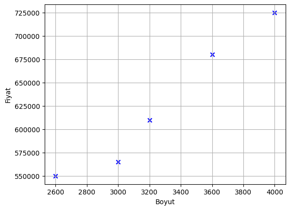
sizes=np.array([2600, 3000, 3200, 3600, 4000]).reshape((-1,1))
prices =np.array([550000, 565000, 610000, 680000, 725000]).reshape((-1,1))
sizes.shape, prices.shape
((5, 1), (5, 1))
plt.scatter(sizes, prices, marker='x', color='b')

plt.xlabel('Boyut')
plt.ylabel('Fiyat')

plt.grid(True)
plt.show()
Lineer regresyon
from sklearn import linear_model
#model
reg = linear_model.LinearRegression()

# modeli verilerle eğitme
reg.fit(sizes,prices)
reg.predict([[3300]])
array([[628715.75342466]])
# theta_0 değeri
reg.intercept_
array([180616.43835616])
# theta_1 değeri
reg.coef_
array([[135.78767123]])
theta_0 = reg.intercept_[0]
theta_1 = reg.coef_[0,0]
# dolayısıyla tahmin fomulu
f=theta_0+theta_1*sizes
f=theta_0+theta_1*3300
f
628715.7534246575
# tum veri setini tahmin etmek için
prices_pred = reg.predict(sizes)
from sklearn.metrics import mean_squared_error, mean_absolute_percentage_error
print("Ortalama kare hatası: ", mean_squared_error(prices, prices_pred))
print("Ortalama mutlak yüzde  hatası: ", mean_absolute_percentage_error(prices, prices_pred))
    Ortalama kare hatası:  186815068.4931509
    Ortalama mutlak yüzde  hatası:  0.019201242020345188
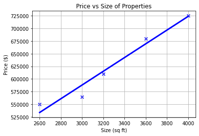
plt.scatter(sizes, prices, marker='x', color='b')

plt.xlabel('Size (sq ft)')
plt.ylabel('Price ($)')
plt.title('Price vs Size of Properties')
plt.plot(sizes, prices_pred, color='blue', linewidth=3)
plt.grid(True)
plt.show()