Yakıt Verimliliği Çalışması
Bu çalışmada yakıt verimliliği ile aşağıdaki sayfada verilen eğitim üzerine çalışmalar yapılmıştır.
https://www.tensorflow.org/tutorials/keras/regression
Veri setini indirmek için tıklayınız.
import matplotlib.pyplot as plt
import numpy as np
import pandas as pd # pip install pandas
import tensorflow as tf
from tensorflow import keras
from tensorflow.keras import layers
column_names = ['MPG', 'Cylinders', 'Displacement', 'Horsepower', 'Weight',
                'Acceleration', 'Model Year', 'Origin']
dataset=pd.read_csv("auto+mpg/auto-mpg.data", names=column_names, na_values='?',
                   comment='\t', sep=' ', skipinitialspace=True)
dataset
| MPG | Cylinders | Displacement | Horsepower | Weight | Acceleration | Model Year | Origin | |
|---|---|---|---|---|---|---|---|---|
| 0 | 18.0 | 8 | 307.0 | 130.0 | 3504.0 | 12.0 | 70 | 1 |
| 1 | 15.0 | 8 | 350.0 | 165.0 | 3693.0 | 11.5 | 70 | 1 |
| 2 | 18.0 | 8 | 318.0 | 150.0 | 3436.0 | 11.0 | 70 | 1 |
| 3 | 16.0 | 8 | 304.0 | 150.0 | 3433.0 | 12.0 | 70 | 1 |
| 4 | 17.0 | 8 | 302.0 | 140.0 | 3449.0 | 10.5 | 70 | 1 |
| ... | ... | ... | ... | ... | ... | ... | ... | ... |
| 393 | 27.0 | 4 | 140.0 | 86.0 | 2790.0 | 15.6 | 82 | 1 |
| 394 | 44.0 | 4 | 97.0 | 52.0 | 2130.0 | 24.6 | 82 | 2 |
| 395 | 32.0 | 4 | 135.0 | 84.0 | 2295.0 | 11.6 | 82 | 1 |
| 396 | 28.0 | 4 | 120.0 | 79.0 | 2625.0 | 18.6 | 82 | 1 |
| 397 | 31.0 | 4 | 119.0 | 82.0 | 2720.0 | 19.4 | 82 | 1 |
398 rows × 8 columns
dataset.isna().sum()
MPG             0
Cylinders       0
Displacement    0
Horsepower      6
Weight          0
Acceleration    0
Model Year      0
Origin          0
dtype: int64
# clean data
dataset = dataset.dropna()
dataset
| MPG | Cylinders | Displacement | Horsepower | Weight | Acceleration | Model Year | Origin | |
|---|---|---|---|---|---|---|---|---|
| 0 | 18.0 | 8 | 307.0 | 130.0 | 3504.0 | 12.0 | 70 | 1 |
| 1 | 15.0 | 8 | 350.0 | 165.0 | 3693.0 | 11.5 | 70 | 1 |
| 2 | 18.0 | 8 | 318.0 | 150.0 | 3436.0 | 11.0 | 70 | 1 |
| 3 | 16.0 | 8 | 304.0 | 150.0 | 3433.0 | 12.0 | 70 | 1 |
| 4 | 17.0 | 8 | 302.0 | 140.0 | 3449.0 | 10.5 | 70 | 1 |
| ... | ... | ... | ... | ... | ... | ... | ... | ... |
| 393 | 27.0 | 4 | 140.0 | 86.0 | 2790.0 | 15.6 | 82 | 1 |
| 394 | 44.0 | 4 | 97.0 | 52.0 | 2130.0 | 24.6 | 82 | 2 |
| 395 | 32.0 | 4 | 135.0 | 84.0 | 2295.0 | 11.6 | 82 | 1 |
| 396 | 28.0 | 4 | 120.0 | 79.0 | 2625.0 | 18.6 | 82 | 1 |
| 397 | 31.0 | 4 | 119.0 | 82.0 | 2720.0 | 19.4 | 82 | 1 |
392 rows × 8 columns
dataset_np= dataset.to_numpy()
dataset_np
array([[ 18. ,   8. , 307. , ...,  12. ,  70. ,   1. ],
       [ 15. ,   8. , 350. , ...,  11.5,  70. ,   1. ],
       [ 18. ,   8. , 318. , ...,  11. ,  70. ,   1. ],
       ...,
       [ 32. ,   4. , 135. , ...,  11.6,  82. ,   1. ],
       [ 28. ,   4. , 120. , ...,  18.6,  82. ,   1. ],
       [ 31. ,   4. , 119. , ...,  19.4,  82. ,   1. ]])
from tensorflow.keras.utils import to_categorical

# Son sütunu al (kategori sütunu)
categorical_column = dataset_np[:, -1]
# One-hot encoding
encoded_column = to_categorical(categorical_column)
encoded_column
array([[0., 1., 0., 0.],
       [0., 1., 0., 0.],
       [0., 1., 0., 0.],
       ...,
       [0., 1., 0., 0.],
       [0., 1., 0., 0.],
       [0., 1., 0., 0.]], dtype=float32)
# Orijinal veriyle birleştir
dataset_encoded = np.hstack((dataset_np[:, :-1], encoded_column))
dataset_encoded
array([[ 18.,   8., 307., ...,   1.,   0.,   0.],
       [ 15.,   8., 350., ...,   1.,   0.,   0.],
       [ 18.,   8., 318., ...,   1.,   0.,   0.],
       ...,
       [ 32.,   4., 135., ...,   1.,   0.,   0.],
       [ 28.,   4., 120., ...,   1.,   0.,   0.],
       [ 31.,   4., 119., ...,   1.,   0.,   0.]])
np.set_printoptions(suppress=True, precision=4)
dataset_encoded[-5:,-5:]
array([[82.,  0.,  1.,  0.,  0.],
       [82.,  0.,  0.,  1.,  0.],
       [82.,  0.,  1.,  0.,  0.],
       [82.,  0.,  1.,  0.,  0.],
       [82.,  0.,  1.,  0.,  0.]])
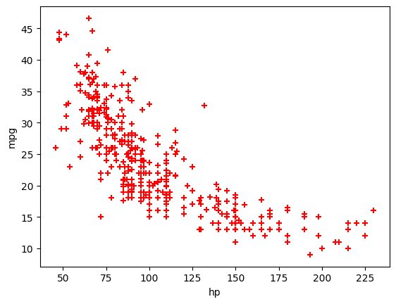
# Horsepower
hp = dataset_encoded[:,3]
mpg = dataset_encoded[:,0]
plt.scatter(hp, mpg, marker="+", color="red")
plt.xlabel("hp")
plt.ylabel('mpg')
plt.show()
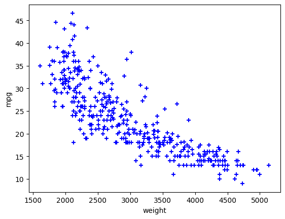
# Horsepower
weight = dataset_encoded[:,4]
mpg = dataset_encoded[:,0]
plt.scatter(weight, mpg, marker="+", color="blue")
plt.xlabel("weight")
plt.ylabel('mpg')
plt.show()
Tek katman, tek nöron
# input ve output
y = mpg  # İlk sütun (çıktı)
X = hp  # Geri kalan sütunlar (girdi)
from sklearn.model_selection import train_test_split
X_train, X_test, y_train, y_test = train_test_split(X, y, test_size=0.2, random_state=42)
from sklearn.preprocessing import MinMaxScaler

# X_train için Min-Max ölçekleme
scaler_X = MinMaxScaler()
# hp
X_train_scaled = scaler_X.fit_transform(X_train.reshape((-1,1)))

# X_test'i aynı scaler ile dönüştür
X_test_scaled = scaler_X.transform(X_test.reshape((-1,1)))

# y_train için Min-Max ölçekleme
scaler_y = MinMaxScaler()
y_train_scaled = scaler_y.fit_transform(y_train.reshape(-1, 1))  # y vektör olduğu için reshape gerekli

# y_test'i aynı scaler ile dönüştür
y_test_scaled = scaler_y.transform(y_test.reshape(-1, 1))
X_train_scaled.shape
(313, 1)
model = keras.models.Sequential([
    layers.Dense(units=1, input_shape=(1,)) # Linear Model
])
model.summary()
Model: "sequential"
_________________________________________________________________
 Layer (type)                Output Shape              Param #
=================================================================
 dense (Dense)               (None, 1)                 2

=================================================================
Total params: 2
Trainable params: 2
Non-trainable params: 0
_________________________________________________________________
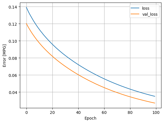
model.compile(optimizer='adam', loss='mse')
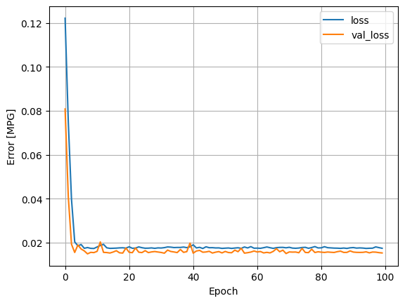
history=model.fit(X_train_scaled, y_train_scaled, epochs=100, validation_data=(X_test_scaled, y_test_scaled))
plt.plot(history.history['loss'], label='loss')
plt.plot(history.history['val_loss'], label='val_loss')
plt.xlabel('Epoch')
plt.ylabel('Error [MPG]')
plt.legend()
plt.grid(True)
plt.show()
y_test_predict_scaled=model.predict(X_test_scaled)
3/3 [==============================] - 0s 3ms/step
y_pred = scaler_y.inverse_transform(y_test_predict_scaled)
y_test[:10]
array([26. , 21.6, 36.1, 26. , 27. , 28. , 13. , 26. , 19. , 29. ])
y_pred[:10]
array([[24.1966],
       [22.6639],
       [24.4965],
       [24.1633],
       [23.6302],
       [23.9967],
       [20.8314],
       [23.9967],
       [23.3303],
       [24.863 ]], dtype=float32)
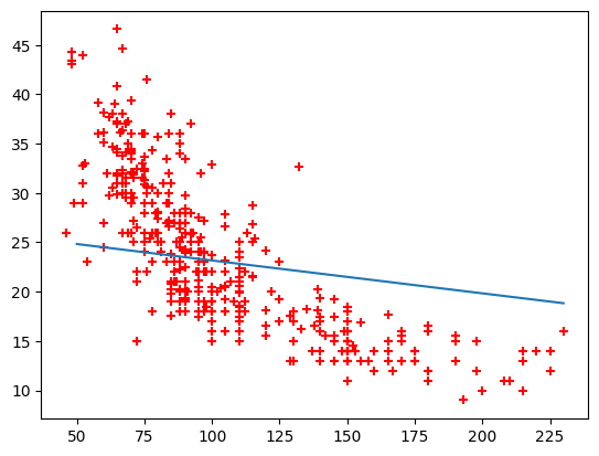
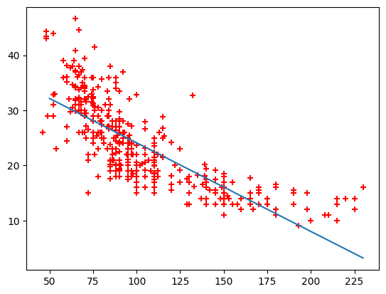
X_line = np.linspace(50, 230, 200).reshape((-1,1))
X_line_scaled = scaler_X.transform(X_line)

y_line_pred_scaled = model.predict(X_line_scaled)

y_line_pred=scaler_y.inverse_transform(y_line_pred_scaled)
7/7 [==============================] - 0s 6ms/step
plt.plot(X_line, y_line_pred)
plt.scatter(hp, mpg, marker="+", color="red")
plt.show()
Aktivasyonsuz büyük model
# DNN
model = keras.Sequential([
    layers.Dense(64,  input_shape=(1,)),
    layers.Dense(64),
    layers.Dense(1)
])
model.compile(loss="mse", optimizer="adam")

model.summary()
Model: "sequential_1"
_________________________________________________________________
 Layer (type)                Output Shape              Param #
=================================================================
 dense_1 (Dense)             (None, 64)                128

 dense_2 (Dense)             (None, 64)                4160

 dense_3 (Dense)             (None, 1)                 65

=================================================================
Total params: 4,353
Trainable params: 4,353
Non-trainable params: 0
_________________________________________________________________
history=model.fit(X_train_scaled, y_train_scaled, epochs=100, validation_data=(X_test_scaled, y_test_scaled))
plt.plot(history.history['loss'], label='loss')
plt.plot(history.history['val_loss'], label='val_loss')
plt.xlabel('Epoch')
plt.ylabel('Error [MPG]')
plt.legend()
plt.grid(True)
plt.show()
y_test_predict_scaled=model.predict(X_test_scaled)
3/3 [==============================] - 0s 3ms/step
y_pred = scaler_y.inverse_transform(y_test_predict_scaled)
y_test[:10]
array([26. , 21.6, 36.1, 26. , 27. , 28. , 13. , 26. , 19. , 29. ])
y_pred[:10]
array([[29.0933],
       [21.6916],
       [30.5413],
       [28.9311],
       [26.3578],
       [28.1282],
       [12.8439],
       [28.1282],
       [24.9084],
       [32.3117]], dtype=float32)
X_line = np.linspace(50, 230, 200).reshape((-1,1))
X_line_scaled = scaler_X.transform(X_line)

y_line_pred_scaled = model.predict(X_line_scaled)

y_line_pred=scaler_y.inverse_transform(y_line_pred_scaled)
7/7 [==============================] - 0s 4ms/step
plt.plot(X_line, y_line_pred)
plt.scatter(hp, mpg, marker="+", color="red")
plt.show()
Aktivasyonlu büyük model
# DNN
model = keras.Sequential([
    layers.Dense(64, activation='relu', input_shape=(1,)),
    layers.Dense(64, activation='relu'),
    layers.Dense(1)
])
model.compile(loss="mse", optimizer="adam")

model.summary()
Model: "sequential_2"
_________________________________________________________________
 Layer (type)                Output Shape              Param #
=================================================================
 dense_4 (Dense)             (None, 64)                128

 dense_5 (Dense)             (None, 64)                4160

 dense_6 (Dense)             (None, 1)                 65

=================================================================
Total params: 4,353
Trainable params: 4,353
Non-trainable params: 0
_________________________________________________________________
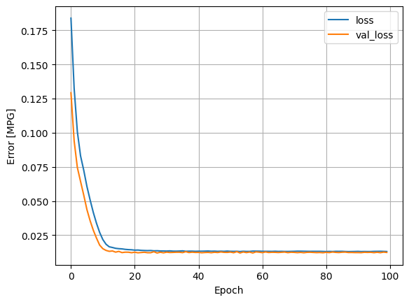
history=model.fit(X_train_scaled, y_train_scaled, epochs=100, validation_data=(X_test_scaled, y_test_scaled))
plt.plot(history.history['loss'], label='loss')
plt.plot(history.history['val_loss'], label='val_loss')
plt.xlabel('Epoch')
plt.ylabel('Error [MPG]')
plt.legend()
plt.grid(True)
plt.show()
y_test_predict_scaled=model.predict(X_test_scaled)
3/3 [==============================] - 0s 9ms/step
y_pred = scaler_y.inverse_transform(y_test_predict_scaled)
y_test[:10]
array([26. , 21.6, 36.1, 26. , 27. , 28. , 13. , 26. , 19. , 29. ])
y_pred[:10]
array([[32.1325],
       [19.3693],
       [34.0669],
       [31.7668],
       [25.9717],
       [29.9602],
       [14.1179],
       [29.9602],
       [22.7098],
       [34.3702]], dtype=float32)
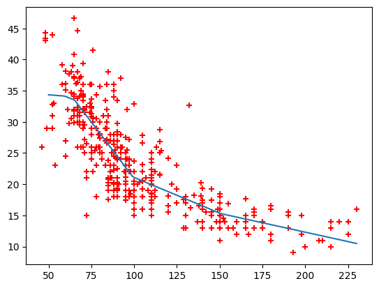
X_line = np.linspace(50, 230, 200).reshape((-1,1))
X_line_scaled = scaler_X.transform(X_line)

y_line_pred_scaled = model.predict(X_line_scaled)

y_line_pred=scaler_y.inverse_transform(y_line_pred_scaled)
7/7 [==============================] - 0s 2ms/step
plt.plot(X_line, y_line_pred)
plt.scatter(hp, mpg, marker="+", color="red")
plt.show()
Çoklu veri
X = dataset_encoded[:,1:]
y = dataset_encoded[:,0]
X_train, X_test, y_train, y_test = train_test_split(X, y, test_size=0.2, random_state=42)
from sklearn.preprocessing import MinMaxScaler

# X_train için Min-Max ölçekleme
scaler_X = MinMaxScaler()
# hp
X_train_scaled = scaler_X.fit_transform(X_train)

# X_test'i aynı scaler ile dönüştür
X_test_scaled = scaler_X.transform(X_test)

# y_train için Min-Max ölçekleme
scaler_y = MinMaxScaler()
y_train_scaled = scaler_y.fit_transform(y_train.reshape(-1, 1))  # y vektör olduğu için reshape gerekli

# y_test'i aynı scaler ile dönüştür
y_test_scaled = scaler_y.transform(y_test.reshape(-1, 1))
X_train_scaled.shape, X_test_scaled.shape, y_train.shape
((313, 10), (79, 10), (313,))
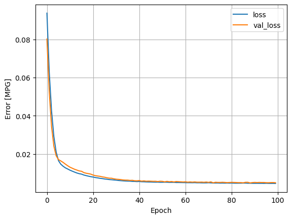
Aktivasyon fonksiyonu olmayan model
model = keras.models.Sequential([
    layers.Dense(units=32, input_shape=(10,)), # Linear Model
    layers.Dense(1)
])
model.summary()
Model: "sequential_4"
_________________________________________________________________
 Layer (type)                Output Shape              Param #
=================================================================
 dense_9 (Dense)             (None, 32)                352

 dense_10 (Dense)            (None, 1)                 33

=================================================================
Total params: 385
Trainable params: 385
Non-trainable params: 0
_________________________________________________________________
model.compile(optimizer='adam', loss='mse')
history=model.fit(X_train_scaled, y_train_scaled, epochs=100, validation_data=(X_test_scaled, y_test_scaled))
plt.plot(history.history['loss'], label='loss')
plt.plot(history.history['val_loss'], label='val_loss')
plt.xlabel('Epoch')
plt.ylabel('Error [MPG]')
plt.legend()
plt.grid(True)
plt.show()
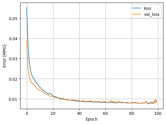
Aktivasyonlu tek katman model
model = keras.models.Sequential([
    layers.Dense(units=32, input_shape=(10,), activation='relu'),
    layers.Dense(1)
])
model.summary()
Model: "sequential_5"
_________________________________________________________________
 Layer (type)                Output Shape              Param #
=================================================================
 dense_11 (Dense)            (None, 32)                352

 dense_12 (Dense)            (None, 1)                 33

=================================================================
Total params: 385
Trainable params: 385
Non-trainable params: 0
_________________________________________________________________
model.compile(optimizer='adam', loss='mse')
history=model.fit(X_train_scaled, y_train_scaled, epochs=100, validation_data=(X_test_scaled, y_test_scaled))
plt.plot(history.history['loss'], label='loss')
plt.plot(history.history['val_loss'], label='val_loss')
plt.xlabel('Epoch')
plt.ylabel('Error [MPG]')
plt.legend()
plt.grid(True)
plt.show()
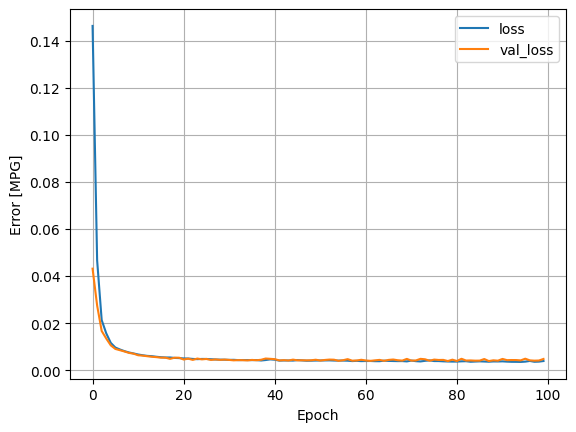
Aktivasyonlu büyük model
model = keras.models.Sequential([
    layers.Dense(units=64, input_shape=(10,), activation='relu'),
    layers.Dense(units=64, activation='relu'),
    layers.Dense(1)
])
model.summary()
Model: "sequential_6"
_________________________________________________________________
 Layer (type)                Output Shape              Param #
=================================================================
 dense_13 (Dense)            (None, 64)                704

 dense_14 (Dense)            (None, 64)                4160

 dense_15 (Dense)            (None, 1)                 65

=================================================================
Total params: 4,929
Trainable params: 4,929
Non-trainable params: 0
_________________________________________________________________
model.compile(optimizer='adam', loss='mse')
history=model.fit(X_train_scaled, y_train_scaled, epochs=100, validation_data=(X_test_scaled, y_test_scaled))
plt.plot(history.history['loss'], label='loss')
plt.plot(history.history['val_loss'], label='val_loss')
plt.xlabel('Epoch')
plt.ylabel('Error [MPG]')
plt.legend()
plt.grid(True)
plt.show()
y_test_predict_scaled=model.predict(X_test_scaled)
3/3 [==============================] - 0s 4ms/step
y_pred = scaler_y.inverse_transform(y_test_predict_scaled)
y_test[:10]
array([26. , 21.6, 36.1, 26. , 27. , 28. , 13. , 26. , 19. , 29. ])
y_pred[:10]
array([[26.7558],
       [22.5017],
       [36.2746],
       [24.9012],
       [29.0538],
       [30.3016],
       [13.2449],
       [30.7193],
       [19.4705],
       [31.5328]], dtype=float32)